Build an internet-of-things dashboard with Google Sheets and RStudio Shiny: Tutorial part 2/3

Dec 27, 2015 · 6 minute read · Comments

This is the second installment of the Shiny + GDocs dashboard tutorial, where we learn how to use a Google Sheet spreadsheet to store data from connected “Internet of Things” data and use Shiny to create a web page to show the data. The first part showed you how to set up a Google Sheet to serve as a data server that accepts POST and GET HTTP requests, as well as how to use pivot tables and filters on the sheets directly. In this section, I’ll walk you through the specific aspects of R that we will wrap in Shiny code. We’ll cover: how to download CSV data from the web, handling date fields, and making various plots with ggplot2. I assume if you are reading tutorial that you already are using R and found the tutorial through a desire to connect to Google Sheets data. If not, I hope this overview will motivate you to learn more R!

If you want to skip to using Shiny, head over to part 3. The finished code files are available on Github: https://github.com/douglas-watson/shiny-gdocs

Chinese translation: https://segmentfault.com/a/1190000004426828

Recommended setup

If you are an experienced R user, you already know what development environment you prefer. Use that one. If not, I recommend RStudio, available for Linux, Mac, and Windows. It has a decent editor (with Vim mode!) and integrates with Shiny. Head over to https://www.rstudio.com/products/rstudio/#Desktop to download it.

You will also need R and the ggplot2. Install R from your package manager on Linux, or download it from here on other platforms: https://www.r-project.org/. Once R and RStudio are installed, open RStudio, and install ggplot2 from the R console:

install.packages('ggplot2')

Import a CSV file from a web URL

Fetching CSV data from the web is trivial: just feed read.csv a url parameter, it automatically downloads the data and makes a data frame with the correct header names. Create a “helpers.R” file, and write the following code in it:

getRaw <- function () {
  data <- read.csv(
    url("https://script.google.com/macros/s/AKfycbxOw-Tl_r0jDV4wcnixdYdUjcNipSzgufiezRKr28Q5OAN50cIP/exec?sheet=Raw"),
    strip.white = TRUE
  )
  data
}

We call the file helpers.R, as it will be used later by the Shiny app. The getRaw function returns a data frame with five variables, named identically to the spreadsheet’s headers:

> data <- getRaw()
> summary(data)
   timestamp                                              date         origin           variable       value      
 Min.   :1.448e+09   Mon Nov 23 2015 22:44:45 GMT+0100 (CET):  4   bedroom:120   humidity   :120   Min.   :23.00  
 1st Qu.:1.448e+09   Mon Nov 23 2015 23:44:45 GMT+0100 (CET):  4   kitchen:120   temperature:120   1st Qu.:23.88  
 Median :1.448e+09   Thu Nov 26 2015 00:44:45 GMT+0100 (CET):  4                                   Median :32.55  
 Mean   :1.448e+09   Thu Nov 26 2015 01:44:45 GMT+0100 (CET):  4                                   Mean   :34.34  
 3rd Qu.:1.448e+09   Thu Nov 26 2015 02:44:45 GMT+0100 (CET):  4                                   3rd Qu.:44.45  
 Max.   :1.449e+09   Thu Nov 26 2015 03:44:45 GMT+0100 (CET):  4                                   Max.   :49.90  
                     (Other)                                :216                                                  
>

Convert date-time column

Let’s now convert the date-time data to a proper R date object. The easiest way is to transform the UNIX timestamp column into a POSIXct object and replace the “date” column. Since we generated UTC dates, we set the time zone to “GMT”. Complete the getRaw function:

getRaw <- function () {
  data <- read.csv(
    url("https://script.google.com/macros/s/AKfycbxOw-Tl_r0jDV4wcnixdYdUjcNipSzgufiezRKr28Q5OAN50cIP/exec?sheet=Raw"),
    strip.white = TRUE
  )
  data$date = as.POSIXct(data$timestamp, tz="GMT", origin="1970-01-01")
  data
}

You’re now ready to rock!

Play with ggplot2

The ggplot2 library provides the brilliant qplot function. A single line of code can produce a huge variety of plots, which makes R my favourite tool to play with data.

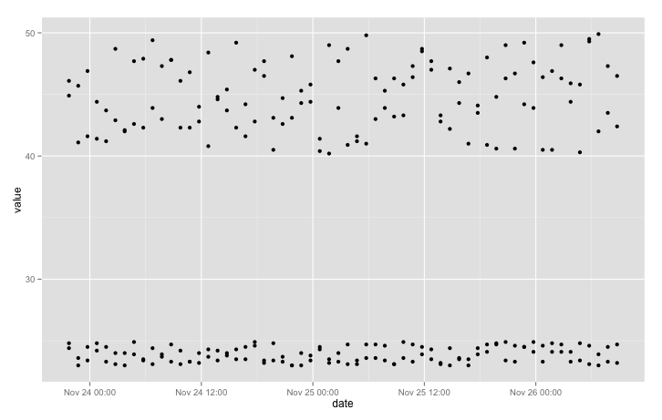
To start off, let’s plot all the values we recorded as a function of time. If you haven’t already, import ggplot2 and helpers.R, and load the CSV data in a data frame.

import(ggplot2)
source("helpers.R")
data <- getRaw()
qplot(date, value, data = data)

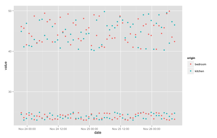
All points on a single plot, a good start, but not very clear.

We can clarify the plot a little by colouring points according to sensor location:

qplot(date, value, data = data, colour = origin)

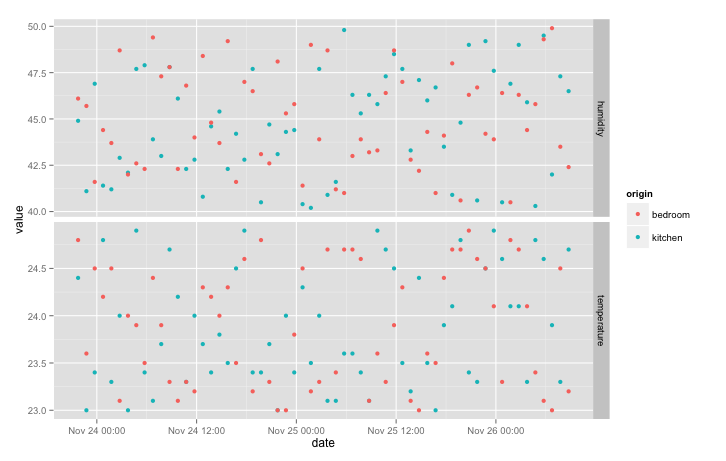
Colouring the points as a function of sensor locations clarifies the plot a bit.

We still can’t distinguish temperature from humidity. Let’s separate those variables into different panels using “facets”. We’ll add the “free_y” option to allow each y to scale independently:

qplot(date, value, data = data, colour = origin) + facet_grid(variable ~ ., scales = "free_y")

Faceted by variable.

Since there is a lot of noise, joining the points with a line makes the plot easier to read:

qplot(date, value, data = data, colour = origin, geom = "line") + facet_grid(variable ~ ., scales = "free_y")

Points replaced by lines

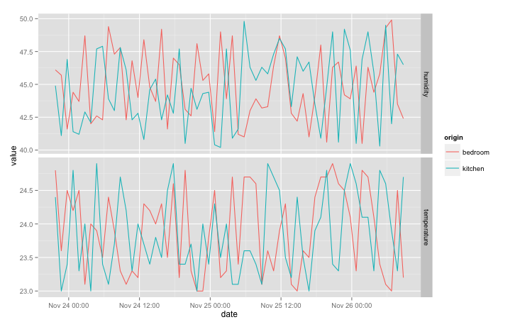
If you add a sensor in a new room, a new line colour will automatically appear on the plot. If you add a new type of data (such as “power” for a power meter), a third facet will appear. Try it! Just modify the Python script to send data from a new location and re-run the python script, the data <- getRaw() line, and the latest qplot instruction.

If the date scale looks wrong, with one tick per point on the x axis, try adding scale_x_datetime:

qplot(date, value, data = data, colour = origin, geom = "line") + scale_x_datetime() + facet_grid(variable ~ ., scales = "free_y")

Other forms of plots.

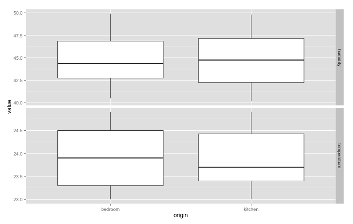
How about box plots to observe variations in temperature and humidity? Easy: just change x axis to “origin”, ditch the colours, and change geometry to “boxplot”:

qplot(origin, value, data = data, geom = "boxplot") + facet_grid(variable ~ ., scales = "free_y")

Box plots are even easier than time series

Have a look at the qplot official documents for more inspiration on plot types: http://docs.ggplot2.org/current

Filtering by date

We’ll cover a final R topic before moving on: filtering data frames, and in particular filtering by date. To filter a data frame, we extract a subset of the data that fulfills a condition. For example, if we want to retrieve all the lines of data that contain a temperature measurement, pick the subset:

data.filt <- subset(data, variable == 'temperature')

Now let’s keep all the data from the second half of our measurement period. Pick a timestamp from the middle of the data frame and create a POSIXct object from it.

ts <- data$timestamp[nrow(data) / 2]
mindate <- as.POSIXct(ts, tz = "GMT", origin = "1970-01-01")

POSIXct objects allow comparisons (> and <), so we can use mindate to filter the data:

data.filt <- subset(data, date > mindate)

Wrapping them in functions for Shiny

For easy access later in Shiny, we’ll just shove the two qplot calls in a function. Our helpers.R file now looks like this, with the library import statement added:

library(ggplot2)

getRaw <- function () {
  data <- read.csv(
    url("https://script.google.com/macros/s/AKfycbxOw-Tl_r0jDV4wcnixdYdUjcNipSzgufiezRKr28Q5OAN50cIP/exec?sheet=Raw"),
    strip.white = TRUE
  )

  data$date = as.POSIXct(data$timestamp, tz="GMT", origin="1970-01-01")
  data
}

timeseriesPlot <- function(data) {
  qplot(date, value, data = data, colour = origin, geom = "line") + scale_x_datetime() + facet_grid(variable ~ ., scales = "free_y")
}

boxPlot <- function(data) {
  qplot(origin, value, data = data, geom = "boxplot") + facet_grid(variable ~ ., scales = "free_y")
}

Douglas Watson